Numpy
Numpy is the core library for scientific computing in Python. It provides a high-performance multidimensional array object, and tools for working with these arrays.
Arrays
A numpy array is a grid of values, all of the same type, and is indexed by a tuple of nonnegative integers. The number of dimensions is the rank of the array; the shape of an array is a tuple of intergers giving the size of the array along each dimension.
Initailize numpy arrays from nested Python lists, and access elements using square brackets:
1 | import numpy as np |
Numpy also provides many functions to create arrays:
1 | import numpy as np |
Array indexing
Numpy offers several ways to index into arrays.
Slicing: Similaer to Python lists, numpy arrays can be sliced. Since arrays may be multidimensional, you must specify a slice for each dimension of the array:
1 | import numpy as np |
You can also mix integer indexing with slice indexing. However, doing so will yield an array of lower rank than the original array:
1 | import numpy as np |
Integer array indexing:When you index into numpy arrays using slicing, the resulting array view will always be a subarray of the original array. In contrast, integer array indexing allows you to construct arbitrary arrays using the data from another array.
1 | import numpy as np |
One usful trick with integer array indexing is selecting or mutating one element from each row of a matrix:
1 | import numpy as np |
Boolean array indexing: Boolean array indexing lets you pick out arbitary elements of an array. Frequently this type of indexing is used to select the elements of an array that satisfy some condition.
1 | import numpy as np |
Datatypes
Every numpy array is a grid of elements of the same type. Numpy provides a large set of numeric datatypes that you can use to construct arrays. Numpy tries to guess a datatype when you create an array, but functions that construct arrays usually also include an optional argument to explictly specify the datatype.
1 | import numpy as np |
Array math
Basic mathematical functions operate elementwise on arrays, and are available both as operator overloads and as functions in the numpy module:
1 | import numpy as np |
Note that unlike MATLAB, * is elementwise multiplication, not matrix multiplication. We instead use the dot function to compute inner products of vectors, to multiply a vector by a matrix, and to multiply matices. dot is available both as a function in the numpy module and as an instance method of array objects:
1 | import numpy as np |
Numpy provides many useful functions for performing computations on arrays; one of the most useful if sum:
1 | import numpy as np |
Apart from computing mathematical functions using arrays, we frequently need to reshape or otherwise manipulate data in arrays. The simplest example of this type of operation is transposing a matrix; to transpose a matrix, simply use the T attribute of an array object:
1 | import numpy as np |
Broadcasting
Broadcasting is a powerful mechanism that allows numpy to work with arrays of different shapes when performing arithmetic operations. Frequently we have a smaller array and a larger array, and we want to use the smaller array multiple times to perform some operation on the larger array.
For example, suppose that we want to add a constant vector to each row of a matrix. We could do it like this:
1 | import numpy as np |
This works; however when the matrix x is very large, computing an explicit loop in Python could be slow. Note that adding the vector v to each row of the matrix x is equivalent to forming a matrix vv by stacking multiple copies of v vertically, then performing elementwise summation of x and vv. We could implement this approach like this:
1 | import numpy as np |
Numpy broadcasting allows us to perform this computation without actually creating multiple copies of v.
Consider this version, using broadcasting:
1 | import numpy as np |
The line y = x + x works even though x has shape (4, 3) and v has shape (3, ) due to broadcasting; this line works as if v actually had shape(4, 3), where each row was a copy of v, and the sum was performed elementwise.
Broadcasting two arrays together follows these rules:
- If the arrays do not have the same rank, prepend the shape of the lower rank array with 1s util both shapes have the same length.
- The two arrays are said to be compatible in a dimension if they have the same size in the dimension, or if one of the arrays has size 1 in that dimension.
- The arrays can be broadcast together if they are compatible in all dimensions.
- After broadcasting, each array behaves as if it had shape equal to the elementwise maximum of the shapes of the two input arrays.
- In any dimension where one array had size 1 and the other array had size greater than 1, the first array behaves as if it were copied along that dimension.
Functions that support broadcasting are known as universal functions. Here are some applications of brodcasting:
1 | import numpy as np |
Numpy Documentation
This brief overview has touched on many of the important things need to know about numpy, but is far from complete. Check out the numpy [numpy reference][http://docs.scipy.org/doc/numpy/reference/] to find out much more.
Matplotlib
Matplotlib is a plotting library. In this section give a brief introduction to the matplotlib.pyplot module, which provides a plotting system similar to that of MATLAB.
Plotting
The most important function in matplotlib is plot, which allows you to plot 2D data. Here is a simple example:
1 | import numpy as np |
Runnig this code produces the following plot:
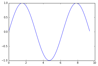
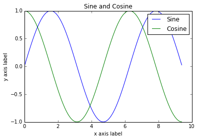
With just a little bit of extra work we can easily plot multiple lines at once, and add a title, legend, and axis labels:
1 | import numpy as np |
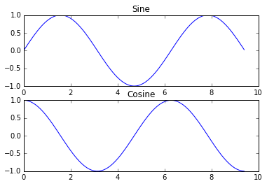
Subplots
You can plot different things in the same figure using the subplot function. Here is an example:
1 | mport numpy as np |
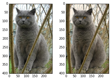
Images
You can use the imshow function to show images. Here is an example:
1 | import numpy as np |
Reference
[Python numpy tutorial][http://cs231n.github.io/python-numpy-tutorial/]
评论